SUMMARY
Since December 2012, during every winter season, the altitude of the zero isochion (snowline) has been determined at the Czech Hydrometeorological Institute for the purposes of operational hydrology. The reason is the estimation of the amount of water stored in snow cover, which is inevitable activity for Czech hydrologists who naturally want their forecasting models to give relevant results. In order to get a better idea about current spatial distribution of snow cover in Czechia, the information on the zero isochion has been extracted from the MODIS imagery coming from the Terra satellite. The obtained time series represents a relatively long period (currently until May 2021), which offers the possibility of analyzing the spatial and temporal dynamics of the zero isochion in Czechia. In this study, the information about the isochion was divided into 27 geomorphological regions and the winter season was divided into the accumulation period and the melting period. The focus was on possible differences between individual regions and time periods, as well as on relationships between zero isochion dynamics and selected factors derived from other geographical data, such as the digital elevation model. Due to different reasons, the data on the isochion were incomplete and did not satisfy the requirements for fitting the models which need regularly/evenly spaced sampling. Therefore, missing daily values were estimated so that the series finally covered the winter seasons from November to May. This was accomplished by the application of a suitable modified EM algorithm that respected both the temporal and the spatial structure of the multivariate time series. Correlation and regression analyses followed, where the main aim was to find out if the belonging to a geomorphological region (with its selected attributes) has an influence, and if there are significant interannual changes.
INTRODUCTION
For more than ten years, the zero isochion has been a practical tool for calculating snow water storage as part of regular hydrological forecast analyses within the Czech Hydrometeorological Institute. The main benefit of determining the isochion is the definition of the areas where we can expect snow cover to be present and where snow cover will be absent, or where we need to take into account snow water equivalent and where it can be neglected. Defining such a boundary within the homogeneous regions of Czechia allows better interpolation of snow cover depth values recorded in the CHMI station network. A more detailed description of hydrological forecast analyses, including the application of the zero isochion in the calculations, is offered by [1, 2]. The content of this paper is related to work [3], where the basic procedures of extracting the zero isochion using satellite images and information on its distribution within the geomorphological regions of Czechia have been summarized. It is the search for correlations and other relationships that can be inferred from the observed series that are the main topic of the following text. One of the key areas of the study is quantifying the degree of dependence of the variability of the average altitude of the zero isochion on the terrain characteristics of the geomorphological regions. The long-term altitude of the zero isochion is analyzed for the entire winter season defined by the months of November to May (for nine years 2013–2021), as well as for parts of the winter season that are typical of snow accumulation, of snow melt and for the rest of this season (for four years 2018–2021). An attempt was made to trace the degree of influence of the factors related to the terrain configuration in different periods of the winter season. Since the length of the collected time series is already quite sufficient (in the sense of an undivided winter season), an equally important task was to see how the altitude of the zero isochion changes with time, i.e., in each year, and whether a significant trend can be observed for some geomorphological regions. In extracting the altitude of the zero isochion and respecting its definition according to [4], a procedure similar to that in [3] was followed for the sake of necessary consistency. New problems were addressed using a variety of statistical techniques, with regression analysis and the selection of significant explanatory variables playing a central role, in addition to descriptive statistics and methods for filling in missing values.
DATA AND METHODOLOGY
Satellite data
A significant portion of the data analyzed in this project comes from the National Snow and Ice Data Center (NSIDC) portal, which supports research on the cryosphere, i.e., snow, ice, glaciers, and frozen ground, as well as the climatic interactions that take place in the cryosphere. The NSIDC administers and distributes scientific data, creates tools for accessing the data, supports data users, conducts scientific research, and educates the public about the cryosphere. As a platform for data originating from the National Aeronautics and Space Administration (NASA), it is also certified as a CoreTrustSeal Regular Member of the World Data System, an interdisciplinary body of the International Science Council (ISC; formerly ICSU). The portal has been distributing data free of charge to the entire scientific community since 1976 in a variety of formats known in the field of RS and in sizes ranging from small text files to terabytes of data. Further information on products, tools and published outputs can be found at [5].
The specific dataset used for the purposes of the zero isochion analysis is designated MODIS/Terra Snow Cover 5-Min L2 Swath 500m, Version 61, and is available, including metadata, from [6]. The name of the dataset contains basic descriptive information about the sensed data. The images are collected using the Moderate Resolution Imaging Spectroradiometer (MODIS) sensor installed on the Terra satellite. Terra is a NASA multinational scientific research satellite in a Sun-synchronous orbit around the Earth that makes simultaneous measurements of the Earth’s atmosphere, soil, and water to contribute to the understanding of how the Earth is changing and to identify implications for life on Earth [7]. The location of the MODIS sensor on the Terra satellite is shown in Fig. 1.
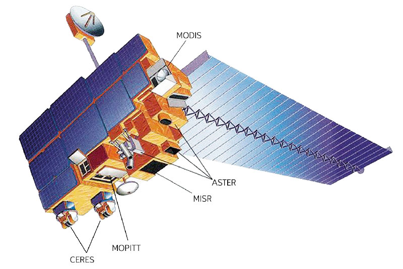
Fig. 1. Terra satellite, launched 18th December 1999 (orbit height: 713 km; orbital velocity: 7,503 km.s-1; maximum velocity: 27,010 km.h-1) and the position of the MODIS sensor (source: [8])
The images tagged with the MOD10_L2 identifier provide information about the snow cover in daily steps. Detection is done using the Normalized Difference Snow Index (NDSI). Another product is a series of correction images that are designed to mitigate errors and mark the detection of uncertain snow cover. Snow-covered landscapes typically have very high reflectance in the visible bands and very low reflectance for the shortwave infrared bands. The NDSI reveals the magnitude of this difference. Each data granule contains 5 minutes of swath data observed at a resolution of 500 m. Data collection began on 24th February 2000 and data revision is now underway for current version 61, which is expected to be completed in spring 2022.
Satellite data download and processing in a GIS environment
The practical aspect of the processing of these data at the CHMI consists in pre-setting the parameters of the area of interest to a rectangle covering the territory of Czechia. If the acquired image is in intersection with this rectangle, the CHMI staff is informed by e-mail as soon as possible about its availability together with a link to download the given data file. The time of sending the notification depends on the image’s complexity. If the image has many classes, there may be a delay. However, most often notifications are sent within 12 hours after acquisition.
Data is provided in the HDF-EOS2 format and is stored as 8-bit unsigned integers. The Hierarchical Data Format (HDF) allows for efficient storage of large, yet quite diverse data and metadata [9]. For the area of interest covering Czechia, the size of such files is approximately 5-25 MB, reflecting the area and spatial distribution of snow in the landscape. Each HDF file is composed of several parameters, of which the output “NDSI_Snow_Cover” is essential for snow detection as it contains attributes divided into nine classes listed in Tab. 1.
Tab. 1. Classes of the NDSI_Snow_Cover output
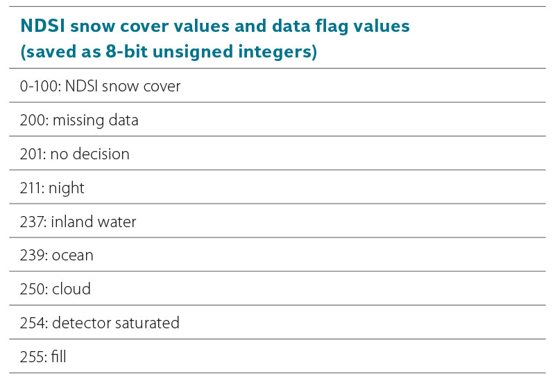
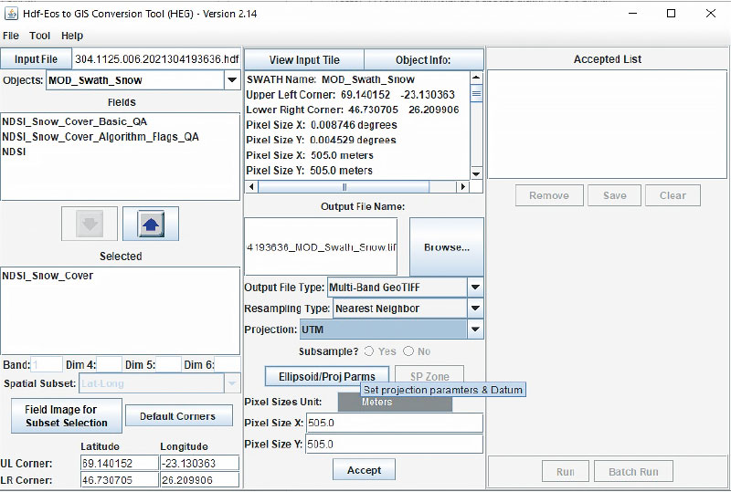
For further work in the GIS environment, it is necessary to extract the individual classes first into a raster form and then into polygons, from which the essential boundary between snow and snow-free areas is exploited. In the first stage of the extraction, it is necessary to use the HEG tool (HDF-EOS To GeoTIFF Conversion Tool), which is freely available as supporting software from the NASA portal [10]. It allows a sufficiently accurate conversion from the HDF format to the GeoTIFF format so that, when projecting to UTM and specifying the corresponding zone (for Czechia 33N or 34N in the east), there is a correct overlay with a Czech Digital Elevation Model (DEM; see below). The local reflections in class 237, i.e., inland water bodies that overlap with the hydrographic base in the GIS (e.g., Rozkoš or Nové Mlýny water reservoirs) are the best verification of the overlay quality. An example of a HEG tool setup is shown in Fig. 2.
Fig. 2. Parameter settings for conversion in the HEG tool
The processing of images in ArcGIS Desktop can be divided into several phases, with the use of each tool adapting to the capabilities of the ArcGIS Desktop license within the CHMI. Future adaptation to newer versions and products can also be expected:
- Extraction of the data of interest from the RS image. The GeoTIFF image is imported with the parameters set in the HEG tool (projection, range). Most often the image is taken in the morning for Czechia, which includes the area from approximately southern Scandinavia to the Alps. In less frequent cases, images with only a partial overlap can also be used, based on the orbital path of the satellite, which may record the territory of Czechia from multiple fly-bys. Images that have an intersection with the preset rectangular mask for Czechia are subjected to cropping to reduce the complexity of the partial calculations. The resulting raster must be first reclassified with respect to the delineation of snow and snow-free areas. The original data up to 2017 were classified more generally into three basic groups: snow, no snow and cloud cover. After 2017, the quality of reflectance from snow cover is broken down in more detail into classes from 0 to 100 (according to the NDSI index), where 0 is a guaranteed snow-free area and 100 is the highest possible reflectance from snow cover. For the purposes of the CHMI hydrology, all snow reflectance values between 1 and 100 are treated as snow in order to provide the largest possible data package for evaluating the zero isochion. As a result, all values 1–100 are reclassified to a value of 50 and values of 0 are treated as snow-free areas. A significant feature based on actual weather conditions is the class value of 201, which is the area of questionable evaluation (NDSI internal calculation), and the class value of 250, which is cloud cover, the most common limiting factor for a full evaluation. The other classes can be considered complementary and can be omitted from further operations. The reclassified raster is further generalized by the Boundary Clean tool to suppress sub-regions of unit pixel sizes, and then the classes are colour coded to make the primary visual overview of the dataset stand out. For further operations, it is necessary to first convert the raster layer to a polygon layer and then to a line layer using the Feature to Line tool. This creates a dataset of lines that have a specific gridcode according to the original raster they surrounded. Specifically, at the contact of two polygons, where one comes with the value of 0 (no snow) and the other with a value of 50 (snow), two lines will be created, one with gridcode 0 and the other with gridcode 50. The element being searched for is then the layer created by the intersection of the selections (Intersect tool) of these two lines and contains all visible boundaries between the snow and no-snow areas. This discontinuous line bounding the recorded snow cover can be referred to as the zero isochion. This line already provides some spatial idea of the position of the snow boundary within the Czech territory. For a more detailed indication of the position, it is necessary to find the approximate value of the altitude at which this line is located. Pixel extraction using a mask was chosen as the simplest method where the isochion line is considered the mask. This is how the altitude values are extracted from the raster base, which is a DEM with a resolution of 25 m (see below).
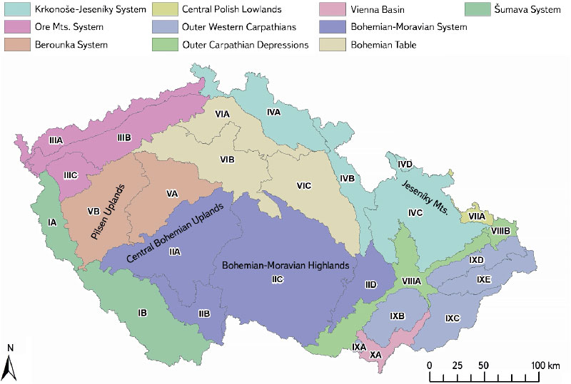
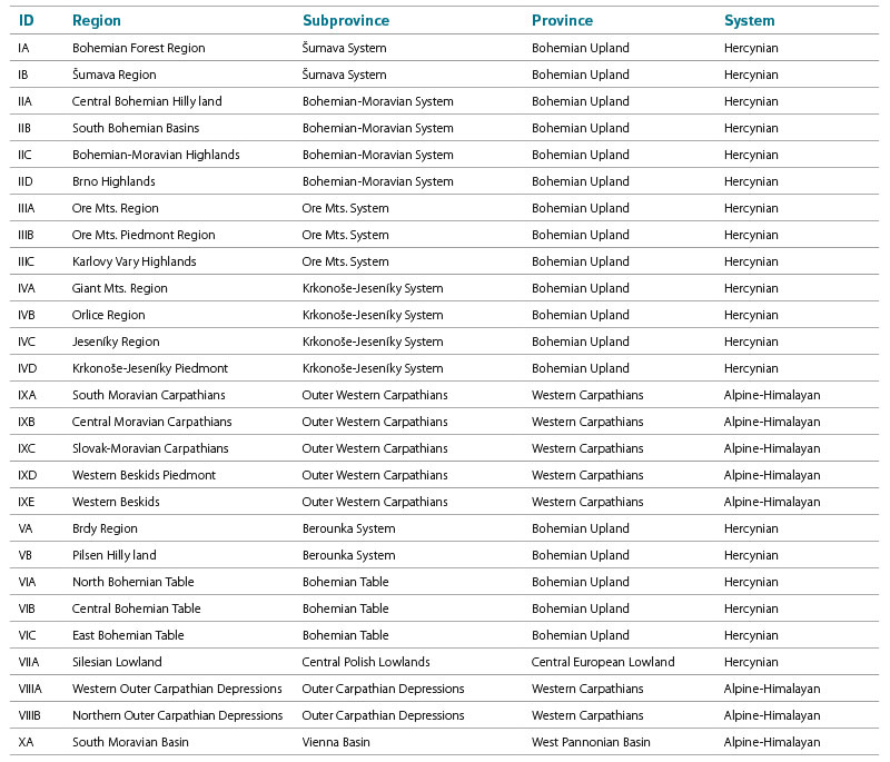
- Spatial data analysis. Geomorphological regions were chosen as the most appropriate division of the Czech territory for the definition of the zero isochion. These areas best reflect the relief features, relative and absolute ruggedness (mountains/lowlands) and the distribution of slope orientation to the cardinal directions (north/south, west/east), i.e., factors that are expected to have a major influence on snow cover accumulation and melting. Within Czechia, there are 27 such treatment regions (see Tab. 2 and Fig. 3 for details). For each of these regions, the extracted set of pixels belonging to the given geomorphological region is evaluated using the Zonal Statistics as Table tool, and the output is a statistic containing information on the number of pixels, their minimum and maximum values, the range of values, the sum of values and, above all, the average value, which is the item that is processed subsequently. The vector layer with geomorphological regions replaces the function of the zero isochion position database, as a column of values is created for each day analyzed, where each geomorphological region is assigned an average position value if it was recorded on that day. The Join Field tool is used to link the statistical output to the region layer attribute table.
- Visual interpretation of data. Visualization of the values can be done by showing labels with these values for each region, possibly with an underlying choropleth map. The situation where an average value is defined for each or at least for most of the geomorphological regions is rather rare during observations, as the cloud factor is often present and in the absence of cloud cover the snow is either limited to mountain areas or, on the contrary, covers the whole territory of Czechia. As mentioned above, the snow boundaries are based on different NDSI reflectance index intensities and each of the average values needs to be critically analyzed (i.e., validated) to see if it is an objective value and can represent the conditions in the region. The evaluation is based not only on internal snow cover data coming from the CHMI observation network (automatic stations, observers, field measurements), but also, for example, on web camera outputs or historical correlations between regions. The position of the zero isochion enters the snow water storage calculation as a limiting value for the spatial interpolation of snow cover parameters, where a fictitious network of zero points is generated for each of the regions, which prevents the interpolation from estimating a non-zero (positive) snow cover depth or snow water equivalent below this position. For this analysis in a GIS environment, the ClidataGIS tool is used, which allows the import of measured data, a more detailed visual inspection, and the setting of parameters for interpolation. The final output is a map, including a supplementary table reflecting changes in snow occurrence over the previous weeks, which is posted on the CHMI portal, and the public can see the predicted water volume in the sub-basins of interest (water reservoirs, major outlet sections of watercourses). Currently, such an output, based on Monday’s measured values, is generated once a week, on Tuesday. In the future, however, it will be possible to produce similar analyses more frequently during the week thanks to the automated network of snow gauging stations combined with satellite imagery.
Fig. 3. Geomorphological regions (for ID see Tab. 2) and their parent subprovinces in Czechia (adapted from [11])
Tab. 2. Geomorphological regions for which, in the winter season, the CHMI determines the average altitude of the zero isochion, and their identifiers (adapted from [11])
Basic geographical material for obtaining terrain explanatory variables
The spatial (but also temporal) variability of the altitude of the zero isochion is influenced by the terrain configuration. Temporal variability will certainly be more related to the climatic conditions of the territorial units for which the study is conducted. Since these territorial units were geomorphological regions for the above-mentioned reasons, it was necessary to obtain a vector layer with polygons representing these regions. This was downloaded from the Geoportal of the Czech Office for Surveying, Mapping and Cadastre, where it is part of the Data200 database (specifically the Description layer) [12]. This layer is based on the geomorphological division described in publication [11], which in fact refers to 28 regions. However, at the CHMI, only 27 regions are traditionally considered, as the Záhorská Lowland is merged with the South Moravian Basin (row with ID XA in Tab. 2). The layer of geomorphological regions has been adjusted accordingly before further analyses.
The Digital Elevation Model (DEM) in the form of a raster, which was the source of information on elevation and other terrain parameters in the geomorphological regions, is based on the Digital Model of Territory prepared at a scale of 1 : 25,000 (DMU 25), which the CHMI purchased from the Military Geographical and Hydrometeorological Office in 2001. This raster with square cells representing an areas of 252 m was created from the original data directly at the CHMI, and contour lines were essential for its creation. The DEM was thus created by suitable interpolation in the then S-42 system. However, because the CHMI switched over time to the UTM zone 33/34N system, the raster was reprojected and resampled into this system (more precisely only zone 33). Similarly, the geometry of the polygon layer of the geomorphological regions was transformed to the UTM zone 33N system.
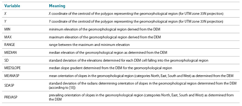
Using the polygon and raster layers, several terrain features were then extracted for each geomorphological region. These were to serve as explanatory variables in the planned regression analysis. Their list and meaning are presented in Tab. 3. Special attention should be paid to the SDASP indicator, which is not well known in the Czech literature. It is the so-called directional standard deviation expressing the variability of slope orientation in individual regions expressed in radians [13]. The R package circular [14] was used to calculate terrain characteristics related to angles. The vector layer was manipulated during extraction using the R package sf [15], while the raster layer was manipulated using the R package terra [16].
Tab. 3. Characteristics of geomorphological regions of Czechia obtained as explanatory variables for next regression analysis
Statistical processing of the extracted data on the altitude of the zero isochion
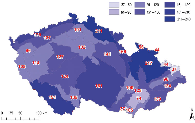
Fig. 4 reveals how many values of zero isochion altitude were available in the original database from December 2012 to May 2021, when the CHMI staff had already evaluated the data completely on their own. Naturally, zero isochion altitude information was only available for the winter seasons, which are usually divided into two calendar years. However, this division is not very suitable for further processing of the time series, so winter seasons were next assigned to years with a larger proportion of months. As the winter season was considered to be November to May, the months of November and December were assigned to the following calendar years. As a result, the winter seasons could be analyzed for the period 2013–2021, i.e., for nine years. For various reasons described earlier, the original database was not complete for the individual geomorphological regions, and even the equidistant weekly step was not followed, since, for example, due to cloud cover, one of the following cloud-free days of the week had to be selected. Missing values and not keeping the same time step make such data quite problematic for subsequent statistical processing, since the vast majority of statistical models require completeness and constancy of the time step (especially when time series models are involved). Although models for this type of data are also being developed (e.g., [17]), it is generally recommended to get rid of their above-mentioned shortcomings so that traditional models can be applied. Finally, the database of zero isochion altitude values was supplemented with estimated values to produce a time series in a daily time step for each geomorphological region that represented all winter seasons of the period 2013–2021 without any missing values. This result was achieved by means of a modified Expectation-Maximization (EM) algorithm that treats the incomplete time series as a multivariate series, where a vector of univariate series with relationships between them is thus considered, while a spline method is applied to all its elements as a filter.
Fig. 4. Total number of days (values) with the detected zero isochion for all winter seasons 2013–2021
The algorithm is described in much more detail in [18], and the same authors implemented it in the R package mtsdi [19], whose mnimput function was also used to fill in the missing daily values.
The daily values were then aggregated for each year (i.e., winter season) using an alpha-trimmed mean to avoid sensitivity to extremes (see, e.g., [20] for more details on its properties). 10% of extreme values were trimmed. In addition, for those years where it was possible, the values were aggregated to represent, in addition to the complete season (labelled as COMPLETE), the different stages of the winter seasons (i.e., ACCUMULATION, MELT and the indistinguishable REST between accumulation and melting). For the definition of the accumulation and melting periods, respectively, the evolution of the snow cover in the border mountains, especially in the Giant Mountains and the Jizera Mountains, was used as a reference. Possible overlaps of these periods caused by possible thawing were not taken into account. However, the different durations of the different seasons in different years were guaranteed. Then, aggregation over all years was also carried out to obtain “long-term” values as explained variables for the regression models to be prepared. The dates defining the periods of snow accumulation and snowmelt were naturally not the same in all years, and therefore the procedure was strictly based on what was observed by a combination of satellite imagery and field survey. For the MELT period, the date of its start was not available for several geomorphological regions and was therefore replaced by the last date of the REST period. Period overlaps were not considered, rather the longer nature of the period was targeted.
For several reasons, including the amount of data obtained, determined by the number of geomorphological regions, a linear model (multivariate additive with parameter estimation using ordinary least squares) and a random forest model were finally chosen for the regression analysis itself. In the former case, terrain explanatory variables were selected based on the Akaike Information Criterion (using a combination of forward and backward variable selection; see [21, 22] for details). Specifically, the selection of explanatory variables was done through the stepAIC function implemented in the R package MASS, which is part of [23]. Before applying the linear models, the possible collinearity between the proposed explanatory variables was specifically investigated using Pearson correlation coefficients. In the case of random forests, the forward feature selection algorithm was applied using the ffs function implemented in the R package CAST [24–26], which mainly needs the R packages caret [27, 28] and randomForest [29] to make it work.
To determine whether a significant interannual monotonic trend can be observed in the altitude of the zero isochion, the non-parametric Mann–Kendall test was applied to each geomorphological region. Since this test, despite its non-parametric nature, is sensitive to autocorrelation in the time series, its trend-free pre-whitening (TFPW) modification implemented in the R package zyp [30] was chosen for the COMPLET series (2013–2021). The theoretical foundations of this test modification can be studied in references [31–33]. Other parts of the winter periods could not be studied in this way because the obtained time series were very short.
RESULTS AND DISCUSSION
Fig. 4. shows the total number of zero isochion altitude values that have been derived from MODIS imagery for each of the 27 geomorphological regions used in the CHMI hydrology practice. A total of 3,216 such values were available for the period December 2012 to May 2021, which amounts to about 6.24% of the theoretically complete daily values (considering all winter seasons contained in the period November 2012 to May 2021, i. e., 51,570 values). This is not solely due to the fact that CHMI hydrologists traditionally focus on obtaining only one value per week for each region, but also because some regions are affected by cloud cover much more frequently than others. At the same time, it should be noted that lowland areas are much less likely to experience snowfall than areas characterised by more mountainous relief. In Fig. 4, this fact is highlighted by the method of a pseudo choropleth map, where geomorphological regions are classified into groups characterised by different intensities of blue. The difference, which is certainly due to the typical altitude or ruggedness within the regions, is very visible. In addition to the above, it must be taken into account that, in terms of spatial and temporal ocurrence of snow cover, the winters of the previous five years can be judged to have been below average, as can be seen from the continuous statistics [2].
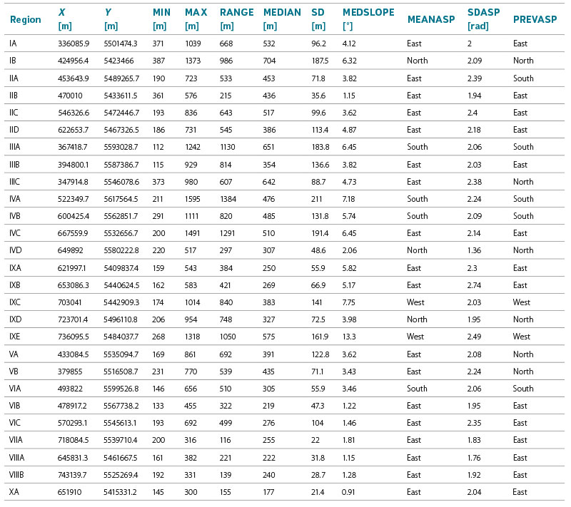
Tab. 4 presents results regarding the extraction of selected terrain variables that were hypothesized to explain the spatial variation in the altitude of the zero isochion and, therefore, to be relevant for the construction of regression models. The list of variables that can be derived from the DEM in this way is certainly not exhaustive, but it was assumed to represent at least the most important factors related to latitude, longitude, and mean, minimum and maximum elevation, terrain ruggedness and slope gradient as well as the slope orientation to the cardinal directions. Particularly important here are the characteristics relating to the variability of elevation, but also the orientation of the slopes to the cardinal directions. The indicators related to slope orientation could have been expressed in angles, but in the end, it was decided that they would enter the regression models as categorical variables resulting from reclassification, since it is not easy to account for angular variables in such models and a transformation is recommended here anyway, usually by applying trigonometric functions.
Tab. 4. Values of selected explanatory variables related to terrain of the 27 geomorphological regions of Czechia
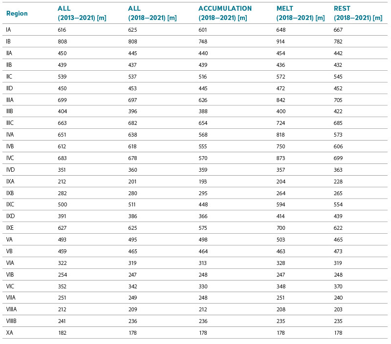
Tab. 5 provides at least a basic idea of the long-term (or rather longer-term) values of the zero isochion altitude in the territory of individual geomorphological regions of Czechia. In addition, Tab. 5 shows how these long-term characteristics vary according to the different stages of the winter season (i.e., accumulation, melting and middle periods when accumulation or melting cannot be distinguished), at least for the years 2018–2021. It should be noted that the full (completed) multivariate series could also include values greater than the maximum and less than the minimum elevation occurring in the geomorphological regions due to extrapolations, which occurred for 16 regions in the supplemented data (in other words, for 1.3% of the total daily values). However, this was not an obstacle when subsequently using the models to identify which terrain features influence the variability of zero isochion altitude. Moreover, these values could be considered realistic if, for example, the highest parts of the regions reached the estimated positions. It is also assumed that these situations were reduced by applying the alpha-trimmed mean.
Tab. 5. Long-term averages of the zero isochion altitude for winter seasons (November–May) for the 27 geomorphological regions of Czechia
Before applying linear models, it is recommended to pay particular attention to the likely collinearity between the explanatory variables, i.e., the phenomenon where two or more variables provide very similar information. Fig. 5 shows through Pearson correlations that, despite the incomplete list of terrain variables, collinearity was very likely present in the set of explanatory variables. In particular, we note a very close correlation (and statistically significant correlation at the 0.05 level) between the elevation maximum and the range between minimum and maximum. Furthermore, a very close relationship between the two variables related to slope orientation can be observed. For these reasons, the range between maximum and minimum elevation and the prevailing slope orientation were not further accounted for in the linear models. An alternative (while retaining all available explanatory variables) could be regression models in which the explanatory variables are principal components instead of the original variables (see, e.g. [34]). For the random forest models, all obtained terrain explanatory variables were deliberately retained before selection. Let us also note that for the random forest models, the original parameter settings were retained as, e.g., in [35].
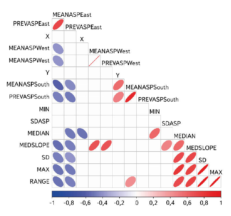
Fig. 5. Pearson correlations between the selected terrain explanatory variables (only correlations significant at the 0.05 level are shown by ellipses and colours)
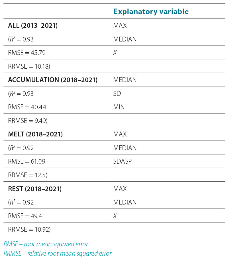
Tab. 6 and 7 already reveal which terrain variables were specifically selected for the linear models (using the Akaike Information Criterion) and random forest models (using the forward feature selection algorithm of [25]), respectively. It can be seen that linear models are much more complex in terms of the inclusion of explanatory variables. Some variables are not significant according to the t statistic, but still contribute to the significance of the whole models. These are even significant at levels smaller than 0.05 according to the F statistic. Also, the values of the coefficients of determination (R2) clearly indicate that the explanation of the variability of the long-term altitude of the zero isochion is more than good here. At the cost of reducing R2 values, the algorithm selected fewer explanatory variables in the case of random forest models. Longitude and elevation extremes stand out very often here. The constantly occurring explanatory variable here is the characteristic related to the mean elevation of the geomorphological regions, which confirms the situation in Fig. 4. Characteristics associated with the variance of elevation (in the case of accumulation) and slope orientation (in the case of melting) also seem to be important for the snow accumulation and snowmelt periods, which sounds quite logical. It should be noted, however, that the random forest is a model based on resampling techniques, so a different run of the algorithm may result in a slightly different choice of variables. Nevertheless, we believe that even so, these selections would be very similar. For example, for snowmelt, the variance of slope orientation related to favourable or unfavourable conditions during the daylight hours will be important.
Tab. 6. Best linear models according to the Akaike Information Criterion
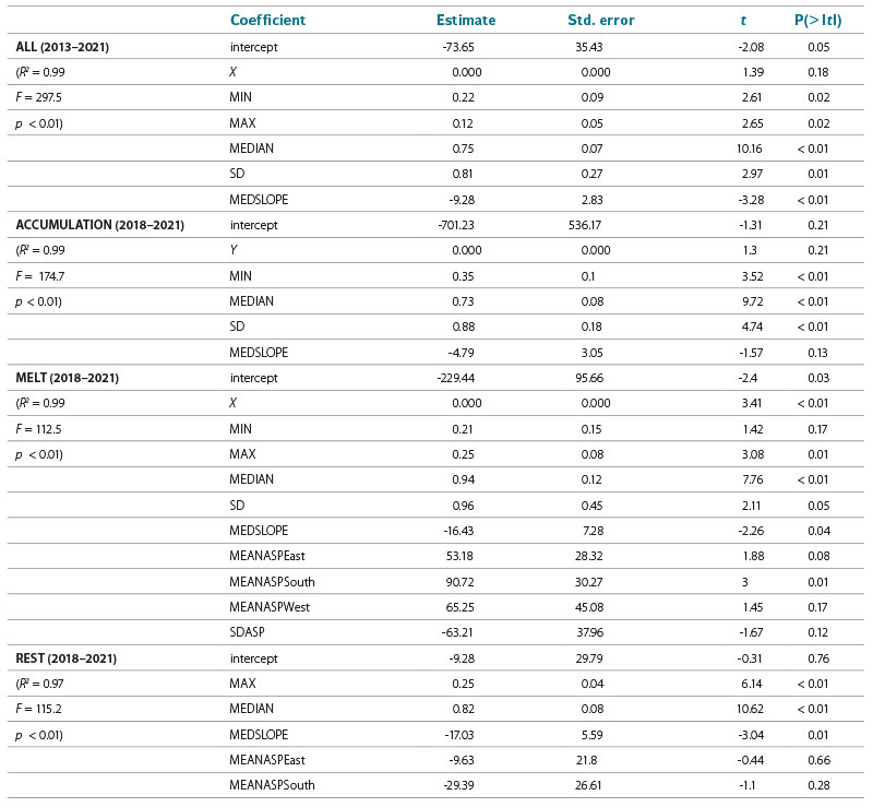
Student t-distribution quantile; P – probability; F – Fisher-Snedecor F-distribution quantile; p – p-value
Tab. 7. Explanatory variables selected by the algorithm according to [25] for random forest models
The analysis of trends, and thus interannual temporal variability of zero isochion altitude, was conducted only for the longest time series, designated as ALL, because the four-year period for which a phase-by-phase distribution discriminating between snow cover gains and losses is available cannot yet be considered representative for this type of analysis. It is clear from Tab. 8 that the zero isochion was rather stable during the 2013–2021 winter seasons. Nevertheless, it is possible to note that five regions are likely to experience a decrease (Ore Mts. Piedmont Region, Central Bohemian Table, Northern Outer Carpathian Depressions, South Moravian Basin) or an increase in zero isochion altitude (Krkonoše-Jeseníky Piedmont). The reasons for such trends may vary from actual increases or decreases in snow cover to the fact that the data for some of these regions may not have been sufficient. For example, from Fig. 6, where the black line shows the time series for only the regions with a significant monotonic trend, it is clear that at least three of these results are quite implausible. Situations where R2 = 1 almost never occur. Moreover, the courses of these suspect series show almost no variability (e.g., the black lines are covered by the blue regression lines), suggesting that the EM algorithm may have failed in filling in the missing values, working with only a few observed values that may have been burdened with large uncertainty on top of that. Let us add that while in Fig. 6 the regression lines are constructed using linear models, in Tab. 8 the regression coefficient and the intercept are related to so-called Sen’s non-parametric estimator [36] to compare the results.
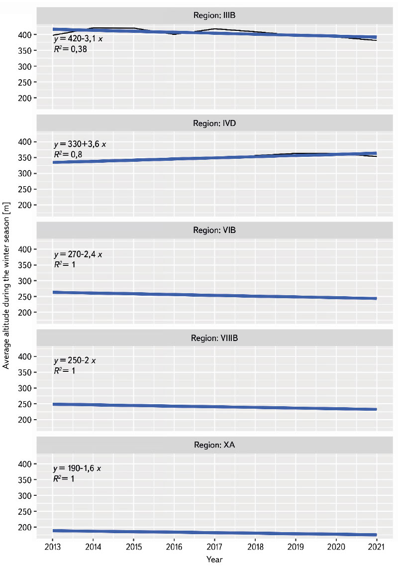
Fig. 6. Course of the annual series of average zero isochion altitude (2013–2021) in five geomorphological regions in Czechia for which a statistically significant monotonic trend was found at the 0.01 level (black line: specific altitude values; blue line: linear trend obtained by the ordinary least squares method)
Tab. 8. Results of trend analysis for all 27 geomorphological regions of Czechia ( : statistically significant increasing trend at the 0.01 level; : statistically significant decreasing trend at the 0.01 level)
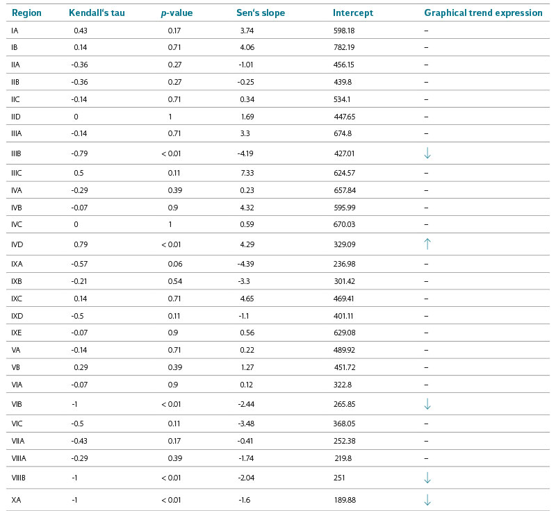
In order to update the table of differences between altitudes of the zero isochion in different geomorphological regions presented in [3], its new version has been compiled (see Tab. 9). It is obvious that the current figures are quite different from those published in the past. For example, there may have been some refinement, where the applied alpha-trimmed mean took the extreme values into account in a different way. Howerver, from the practical point of view of the methodology for calculating snow water storage, the relationship between the mountain border regions where snow cover is longest and most frequent, is the most important for CHMI forecasters. Nevertheless, it is also necessary to mention the risk of significant spring flooding from melting snow, which is more associated with snow cover in the lowlands, i.e., in the tables surrounding the Elbe River. In such situations, the zero isochion is either completely suppressed and snow occurs over the whole territory, or the boundary is quite sharp and delimits the warmest areas and heat islands. Tab. 9 only confirms the experience from the zero isochion analyses, especially the most widely used relationship, namely that between the Giant Mountains Region and the Šumava Region. This can be characterised simply by the fact that the snow cover in the Bohemian Forest always starts 100 metres or more higher as compared with the snowline in the Giant Mountains. The reasons for this can be seen in the ruggedness of the local regions, with the Giant Mountains representing steeper slopes and the Czech part of the Bohemian Forest representing a more gradual transition to lower areas.
Tab. 9. Differences between long-term averages of the zero isochion altitude for winter seasons (November–May) across all 27 geomorphological regions of Czechia (in m)
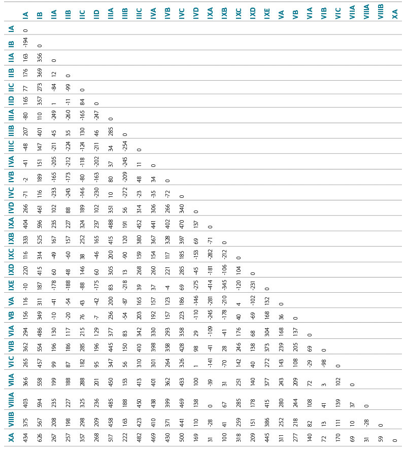
Fig. 7 demonstrates an example of the output obtained with MODIS imagery and it also documents the conditions of snow cover loss in early April 2021. It shows the most common situation where snow cover is present only at the highest elevations of the mountains, where it is also partially covered by clouds. In contrast, the lowlands no longer have snow at all, just as the uncertainly definable areas with snow are no longer present at the end of winter, as characterised by code 201 (see Tab. 1).
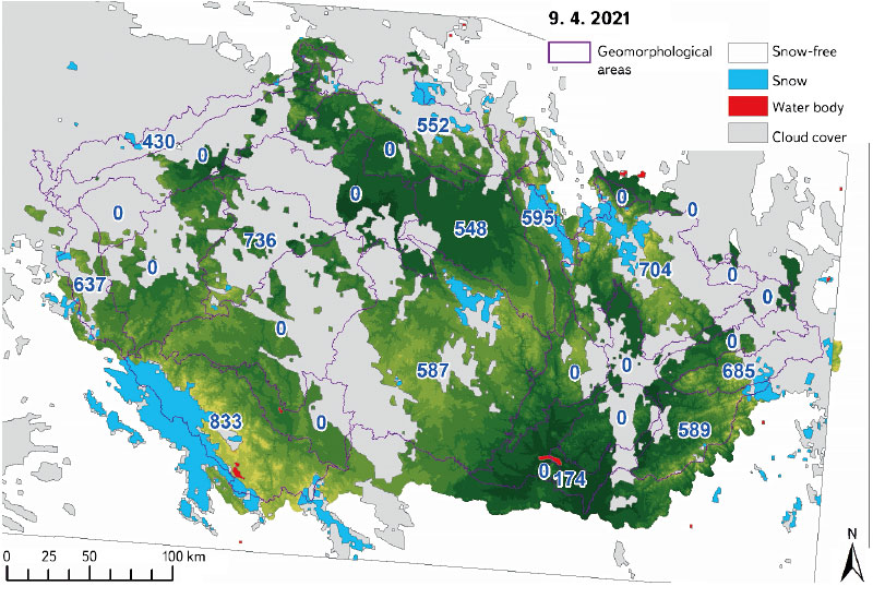
Fig. 7. Analyzed situation on 9th April 2021 where the selected classes from Tab. 1 are depicted above the digital elevation model (values determine the average position of the zero isochion in m a. s. l. and 0 determines the area without recorded zero isochion)
CONCLUSION
This paper presents updated findings concerning the altitude of the zero isochion, i.e., the line representing the boundary between the snow and snow-free areas, in 27 geomorphological regions of Czechia, which are used in hydrological practice of the CHMI for estimating the snow water equivalent. Since snow represents a significant component of runoff in Czechia, this activity is necessary before running hydrological models used at the CHMI for both operational purposes and balance calculations. Field surveys are costly and time-consuming, and do not provide a sufficiently detailed picture of the spatial distribution of snow in regions that are often quite rugged in Czechia. Therefore, satellite imagery has been successfully used to refine this picture, and after appropriate calibration with data collected in the field, it can be very helpful in determining the boundary between snow and snow-free regions (see, e.g., [1] and [37]). The study thus built on previous research and, using an extended time series of zero isochion altitudes to May 2021, sought to answer the questions outlined in the conclusions of [3]. In particular, the spatial variability of the zero isochion altitude was studied and it was examined through regression models which terrain-related factors (determined in a GIS environment from the DEM based on the DMU 25 work) matter most for the variation of the zero isochion. The alpha-trimmed mean calculated from daily values was taken as the representative explained variable here, as it was assumed to reduce the influence of uncertainty in the determination of the position of the zero isochion. Moreover, the average zero isochion altitude in each region represents to some extent a limiting position below which non-zero (positive) values of snow cover depth and hence snow water equivalent can no longer be expected in interpolation processes. Given the uncertainties associated with MODIS imagery, we believe that if the derivation of the zero isochion is appropriately combined with the interpolation of values obtained from ground-based measurements, some of these uncertainties can be reduced to a great extent. Thus, the regression models constructed here to explain spatial variability can be very useful, for example, in estimating the (average) position of the zero isochion in situations where regions are mostly covered by clouds. It has been found that mean but also extreme values of elevation have a large influence. Longitude also seems to play a role. In the case of snow accumulation, the standard deviation calculated from the elevations occurring in a given geomorphological region is added to the explanatory variables in the regression models. In the case of snowmelt, the standard deviation obtained from all angles determining slope orientation appears to be significant. The study of the temporal variability of the zero isochion altitude was carried out by trend analysis in order to determine whether the presence of monotonic deterministic trends can be observed. In order to reduce the influence of autocorrelation, the TFPW modification of the Mann–Kendall test was applied. The results show that snow cover, and hence the zero isochion, behaved stably during the winter seasons. A statistically significant interannual trend was found only in five geomorphological regions. However, the results of the analyses should be interpreted with caution. For example, in three areas the coefficient of determination was suspiciously equal to one, which is a very rare phenomenon. Instead of indicating reality, this fact rather indicates that the Expectation-Maximization (EM) algorithm used to fill in the missing values of the zero isochion altitude failed in some cases. This was due to lack of information, which was certainly caused by the small amount of data obtained from MODIS images or derived products.
As indicated above, revisions to the NDSI index-based product are due to be completed in spring 2022. This could subsequently provide some sort of verification at the CHMI whether the relationships presented in this paper are still valid. Naturally, the deployment of (semi)automatic processing of data coming from MODIS imagery is proposed, provided that the CHMI staff deepen their scripting skills. It is highly recommended to extend the time series towards history, considering that products related to snow detection on the Earth’s surface have been available since 2000. It is also suggested to complement the data considering that MODIS imagery has a much finer time step than one week. This may also allow the application of more sophisticated time series models than simple trend analysis. This will refine the notion of the temporal dynamics of the zero isochion if the explanatory variables also include a number of climatological features along with the terrain characteristics. The explanation for the differences in the position of the zero isochion can also be found in different climatic conditions, especially in the occurrence of rainfall situations, which mainly affect the south-west part of Czechia, while they do not reach such intensities towards the northern mountain ranges anymore. It is also worth looking at other characteristics related to the zero isochion that may enter the models as explanatory variables. For example, the gradient of change of the zero isochion or the change in the duration of the zero isochion presence a certain elevation zone can provide interesting information to hydrologists. Similar variables have already been studied in [38], and especially the period of snow-melt and its effect on runoff was the focus of study [39]. The method by which the zero isochion is extracted in these publications is also worth mentioning. This method differs from the methodology presented here, and therefore a comparison of the two approaches using data for Czechia is naturally offered here.
The spatial resolution of the analyzed grid (500 m) remains a fundamental limitation for a more precise definition of the position of the zero isochion. Thus, spatial refinement, in addition to process automation, is necessary for a deeper implementation of the zero isochion in the calculation of snow water storage. One possibility could be the differentiation of the reclassification of products with NDSI values according to different factors, which has proven to be successful in Austria according to [40]. However, the precondition is that the length of the derivation of the zero isochion will satisfy the requirement of the CHMI operational hydrology to have this result within 24 hours. More accurate spatial data currently exist, but again with a considerable time delay between acquisition and availability. Some promise, in this decade, can be seen in local observing systems or in the European COPERNICUS programme with Sentinel missions (see, e.g., [41]). It will certainly be an equally important task to study the snow cover properties separately for the accumulation, melting and remaining phases of the winter season, because – as the results of this study have shown – this division makes sense.
Last but not least, the question arises whether it is more advantageous to map the snow cover area directly using MODIS imagery. This would only be possible under ideal cloud-free conditions, when an overview of the whole Czech territory, or at least all regions with snow cover, is guaranteed. Such situations are in fact only minimal, on the order of units of days during the season. For this reason, MODIS imagery cannot currently be implemented in snow cover area calculations as a regularly used tool, but only as a supplement to the information obtained from the relatively dense snow gauging network of the CHMI. On the contrary, some potential can be found just in the calibration of the model based on the available zero isochion altitude series and its ability to predict for the “invisible” locations.
Acknowledgements
Both authors are supported within the so-called Long-Term Concept of Development of the Research Organization CHMI. The statistical work of O. Ledvinka is also supported by the Technology Agency of the Czech Republic (project SS01020366 “Using remote sensing to assess negative impacts of rainstorms”). The authors would like to express their gratitude for this support.
The paper has been peer-reviewed.
